Author:
(1) Mingda Chen.
Table of Links
-
3.1 Improving Language Representation Learning via Sentence Ordering Prediction
-
3.2 Improving In-Context Few-Shot Learning via Self-Supervised Training
-
4.2 Learning Discourse-Aware Sentence Representations from Document Structures
-
5 DISENTANGLING LATENT REPRESENTATIONS FOR INTERPRETABILITY AND CONTROLLABILITY
-
5.1 Disentangling Semantics and Syntax in Sentence Representations
-
5.2 Controllable Paraphrase Generation with a Syntactic Exemplar
5.2 Controllable Paraphrase Generation with a Syntactic Exemplar
5.2.1 Introduction
Controllable text generation has recently become an area of intense focus in the NLP community. Recent work has focused both on generating text satisfying certain stylistic requirements such as being formal or exhibiting a particular sentiment (Hu et al., 2017; Shen et al., 2017a; Ficler and Goldberg, 2017), as well as on generating text meeting structural requirements, such as conforming to a particular template (Iyyer et al., 2018; Wiseman et al., 2018).
These systems can be used in various application areas, such as text summarization (Fan et al., 2018a), adversarial example generation (Iyyer et al., 2018), dialogue (Niu and Bansal, 2018), and data-to-document generation (Wiseman et al., 2018). However, prior work on controlled generation has typically assumed a known, finite set of values that the controlled attribute can take on. In this work, we are interested instead in the novel setting where the generation is controlled through an exemplar sentence (where any syntactically valid sentence is a valid exemplar). We will focus in particular on using a sentential exemplar to control the syntactic realization of a generated sentence. This task can benefit natural language interfaces to information systems by suggesting alternative invocation phrases for particular types of queries (Kumar et al., 2017). It can also bear on dialogue systems that seek to generate utterances that fit particular functional categories (Ke et al., 2018).
To address this task, we propose a deep generative model with two latent variables, which are designed to capture semantics and syntax. To achieve better disentanglement between these two variables, we design multi-task learning objectives that make use of paraphrases and word order information. To further facilitate the learning of syntax, we additionally propose to train the syntactic component of our model with word noising and latent word-cluster codes. Word noising randomly replaces word tokens in the syntactic inputs based on a part-of-speech tagger used only at training time. Latent codes create a bottleneck layer in the syntactic encoder, forcing it to learn a more compact notion of syntax. The latter approach also learns interpretable word clusters. Empirically, these learning criteria and neural architectures lead to better generation quality and generally better disentangled representations.

To evaluate this task quantitatively, we manually create an evaluation dataset containing triples of a semantic exemplar sentence, a syntactic exemplar sentence, and a reference sentence incorporating the semantics of the semantic exemplar and the syntax of the syntactic exemplar. This dataset is created by first automatically finding syntactic exemplars and then heavily editing them by ensuring (1) semantic variation between the syntactic inputs and the references, (2) syntactic similarity between the syntactic inputs and the references, and (3) syntactic variation between the semantic input and references. Examples are shown in Fig. 5.3. This dataset allows us to evaluate different approaches quantitatively using standard metrics, including BLEU (Papineni et al., 2002) and ROUGE (Lin, 2004). As the success of controllability of generated sentences also largely depends on the syntactic similarity between the syntactic exemplar and the reference, we propose a “syntactic similarity” metric based on evaluating tree edit distance between constituency parse trees of these two sentences after removing word tokens.
Empirically, we benchmark the syntactically-controlled paraphrase network (SCPN) of Iyyer et al. (2018) on this novel dataset, which shows strong performance with the help of a supervised parser at test-time but also can be sensitive to the quality of the parse predictor. We show that using our word position loss effectively characterizes syntactic knowledge, bringing consistent and sizeable improvements over syntactic-related evaluation. The latent code module learns interpretable latent representations. Additionally, all of our models can achieve improvements over baselines. Qualitatively, we show that our models do suffer from the lack of an abstract syntactic representation, though we also show that SCPN and our models exhibit similar artifacts.
5.2.2 Related Work
We focus primarily on the task of paraphrase generation, which has received significant recent attention (Quirk et al., 2004; Prakash et al., 2016; Mallinson et al., 2017; Dong et al., 2017; Ma et al., 2018b; Li et al., 2018, inter alia).
In seeking to control generation with exemplars, our approach relates to recent work in controllable text generation. Whereas much work on controllable text generation seeks to control distinct attributes of generated text (e.g., its sentiment or formality) (Hu et al., 2017; Shen et al., 2017a; Ficler and Goldberg, 2017; Fu et al., 2018; Zhao et al., 2018, inter alia), there is also recent work which attempts to control structural aspects of the generation, such as its latent (Wiseman et al., 2018) or syntactic (Iyyer et al., 2018) template. Our work is closely related to this latter category, and to the syntactically-controlled paraphrase generation of Iyyer et al. (2018) in particular, but our proposed model is different in that it simply uses a single sentence as a syntactic exemplar rather than requiring a supervised parser. This makes our setting closer to style transfer in computer vision, in which an image is generated that combines the content from one image and the style from another (Gatys et al., 2016). In particular, in our setting, we seek to generate a sentence that combines the semantics from one sentence with the syntax from another, and so we only require a pair of (unparsed) sentences. We also note concurrent work that attempts to use sentences as exemplars in controlling generation (Lin et al., 2020b) in the context of data-to-document generation (Wiseman et al., 2017).
Another related line of work builds generation upon sentential exemplars (Guu et al., 2018; Weston et al., 2018; Pandey et al., 2018; Cao et al., 2018; Peng et al., 2019) in order to improve the quality of the generation itself, rather than to allow for control over syntactic structures.
5.2.3 Model and Training
Given two sentences X and Y , our goal is to generate a sentence Z that follows the syntax of Y and the semantics of X. We refer to X and Y as the semantic template and syntactic template, respectively.
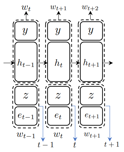
To solve this problem, we adapt the VGVAE model described in Section 5.1. In particular, we assume a generative model that has two latent variables: y for semantics and z for syntax (as depicted in Fig. 5.1)
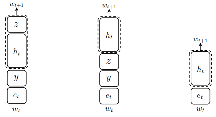
Decoders. As shown in Fig. 5.4, at each time step, we concatenate the syntactic variable z with the previous word’s embedding as the input to the decoder and concatenate the semantic variable y with the hidden vector output by the decoder for predicting the word at the next time step. Note that the initial hidden state of the decoder is always set to zero.
Latent Codes for Syntactic Encoder Since what we want from the syntactic encoder is only the syntactic structure of a sentence, using standard word embeddings tends to mislead the syntactic encoder to believe the syntax is manifested by the exact word tokens. An example is that the generated sentence often preserves the exact pronouns or function words in the syntactic input instead of making necessary changes based on the semantics. To alleviate this, we follow Chen and Gimpel (2018) to represent each word with a latent code (LC) for word clusters within the
word embedding layer. Our goal is for this to create a bottleneck layer in the word embeddings, thereby forcing the syntactic encoder to learn a more abstract representation of the syntax. However, since our purpose is not to reduce model size (unlike Chen and Gimpel, 2018), we marginalize out the latent code to get the embeddings during both training and testing. That is,

Multi-Task Training. Aside from ELBO, we use multi-task training losses: PRL and WPL, as described in Section 5.1.4.
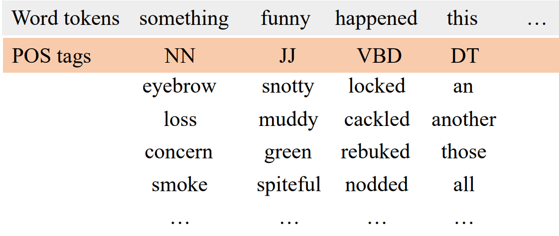
Word Noising via Part-of-Speech Tags. In practice, we often observe that the syntactic encoder tends to remember word types instead of learning syntactic structures. To provide a more flexible notion of syntax, we add word noising (WN) based on part-of-speech (POS) tags. More specifically, we tag the training set using the Stanford POS tagger (Toutanova et al., 2003). Then we group the word types based on the top two most frequent tags for each word type. During training, as shown in Fig. 5.5, we noise the syntactic inputs by randomly replacing word tokens based on the groups and tags we obtained. This provides our framework many examples of word interchangeability based on POS tags, and discourages the syntactic encoder from memorizing the word types in the syntactic input. When using WN, the probability of noising a word is tuned based on development set performance.
5.2.4 Experimental Setup
Training Setup. For training with the PRL, we require a training set of sentential paraphrase pairs. We use ParaNMT, a dataset of approximately 50 million paraphrase pairs. To ensure there is enough variation between paraphrases, we filter out paraphrases with high BLEU score between the two sentences in each pair, which leaves us with around half a million paraphrases as our training set. All hyperparameter tuning is based on the BLEU score on the development set (see appendix for more details). Code and data are available at https://github.com/ mingdachen/syntactic-template-generation.
Evaluation Dataset and Metrics. To evaluate models quantitatively, we manually annotate 1300 instances based on paraphrase pairs from ParaNMT independent from our training set. Each instance in the annotated data has three sentences: semantic input, syntactic input, and reference, where the semantic input and the reference can be seen as human generated paraphrases and the syntactic input shares its syntax with the reference but is very different from the semantic input in terms of semantics. The differences among these three sentences ensure the difficulty of this task. Fig. 5.3 shows examples.
The annotation process involves two steps. We begin with a paraphrase pair <U,V> First, we use an automatic procedure to find, for each sentence u, a syntactically-similar but semantically-different other sentence t. We do this by seeking sentences t with high edit distance of predicted POS tag sequences and low BLEU score with u. Then we manually edit all three sentences to ensure (1) strong semantic match and large syntactic variation between the semantic input u and reference v, (2) strong semantic match between the syntactic input t and its post-edited version, and (3) strong syntactic match between the syntactic input t and the reference v. We randomly pick 500 instances as our development set and use the remaining 800 instances as our test set. We perform additional manual filtering and editing of the test set to ensure quality.
For evaluation, we consider two categories of automatic evaluation metrics, designed to capture different components of the task. To measure roughly the amount of semantic content that matches between the predicted output and the reference, we report BLEU score (BL), METEOR score (MET; Banerjee and Lavie, 2005) and three ROUGE scores, including ROUGE-1 (R-1), ROUGE-2 (R-2) and ROUGE-L (RL). Even though these metrics are not purely based on semantic matching, we refer to them in this paper as “semantic metrics” to differentiate them from our second metric category, which we refer to as a “syntactic metric”. For the latter, to measure the syntactic similarity between generated sentences and the reference, we report the syntactic tree edit distance (ST). To compute ST, we first parse the sentences using Stanford CoreNLP, and then compute the tree edit distance (Zhang and Shasha, 1989) between constituency parse trees after removing word tokens.
Baselines. We report results for three baselines. The first two baselines directly output the corresponding syntactic or semantic input for each instance. For the last baseline, we consider SCPN (Iyyer et al., 2018). As SCPN requires parse trees for both the syntactic and semantic inputs, we follow the process in their paper and use the Stanford shift-reduce constituency parser (Manning et al., 2014) to parse both, then use the parsed sentences as inputs to SCPN. We report results for SCPN when using only the top two levels of the parse as input (template) and using the full parse as input (full parse).
5.2.5 Experimental Results
As shown in Table 5.5, simply outputting the semantic input shows strong performance across the BLEU, ROUGE, and METEOR scores, which are more relevant to semantic similarity, but shows much worse performance in terms of ST. On the other hand, simply returning the syntactic input leads to lower BLEU, ROUGE, and METEOR scores but also a very strong ST score. These trends provide validation of the evaluation dataset, as they show that the reference and the semantic input match more strongly in terms of their semantics than in terms of their syntax, and also that
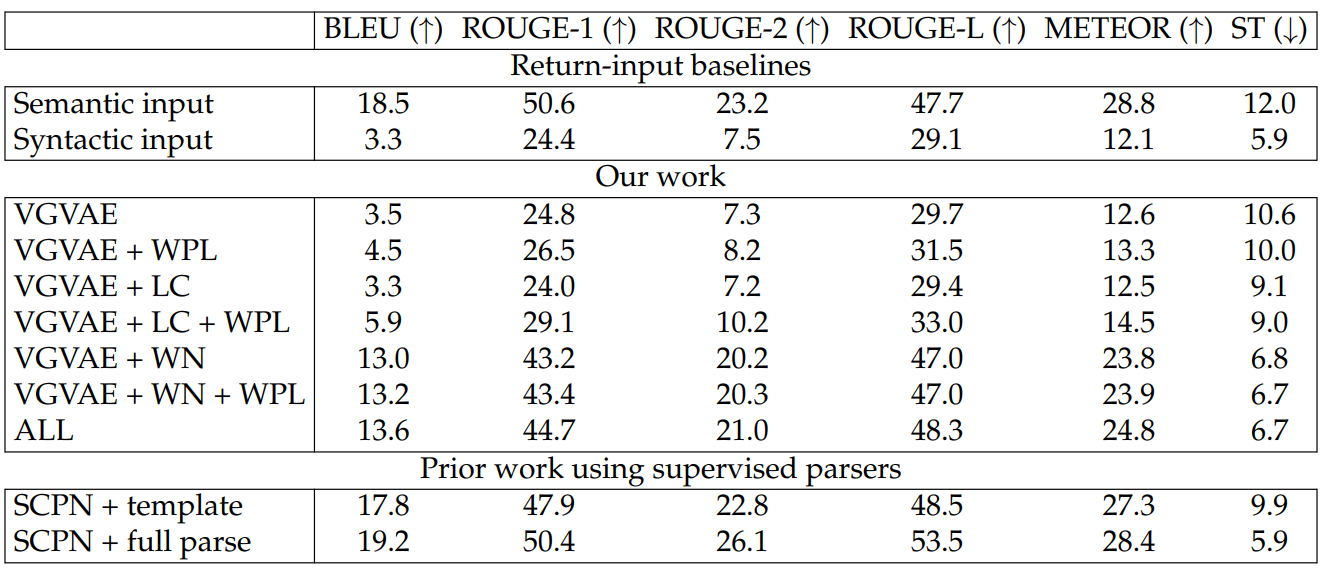
the reference and the syntactic input match more strongly in terms of their syntax than in terms of their semantics. The goal in developing systems for this task is then to produce outputs with higher semantic metric scores than the syntactic input baseline and simultaneously higher syntactic scores than the semantic input baseline.
Among our models, adding WPL leads to gains across both the semantic and syntactic metric scores. The gains are much larger without WN, but even with WN, adding WPL improves nearly all scores. Adding LC typically helps the semantic metrics (at least when combined with WPL) without harming the syntactic metric (ST). We see the largest improvements, however, by adding WN, which uses an automatic part-of-speech tagger at training time only. Both the semantic and syntactic metrics increase consistently with WN, as the syntactic variable is shown many examples of word interchangeability based on POS tags.
While the SCPN yields very strong metric scores, there are several differences that make the SCPN results difficult to compare to those of our models. In particular, the SCPN uses a supervised parser both during training and at test time, while our strongest results merely require a POS tagger and only use it at training time. Furthermore, since ST is computed based on parse trees from a parser, systems that explicitly use constituency parsers at test time, such as SCPN, are likely to be favored by such a metric. This is likely the reason why SCPN can match the syntactic input baseline in ST. Also, SCPN trains on a much larger portion of ParaNMT. We


find large differences in metric scores when SCPN only uses a parse template (i.e., the top two levels of the parse tree of the syntactic input). In this case, the results degrade, especially in ST, showing that the performance of SCPN depends on the quality of the input parses. Nonetheless, the SCPN results show the potential benefit of explicitly using a supervised constituency parser at both training and test time. Future work can explore ways to combine syntactic parsers with our models for more informative training and more robust performance.
5.2.6 Analysis
Effect of Paraphrase Reconstruction Loss. We investigate the effect of PRL by removing PRL from training, which effectively makes VGVAE a variational autoencoder. As shown in Table 5.6, making use of pairing information can improve performance both in the semantic-related metrics and syntactic tree edit distance.
Effect of Position of Word Position Loss. We also study the effect of the position of WPL by (1) using the decoder hidden state, (2) using the concatenation of word embeddings in the syntactic encoder and the syntactic variable, (3) using the concatenation of word embeddings in the decoder and the syntactic variable, or (4) adding it on both the encoder embeddings and decoder word embeddings. Table 5.7 shows that adding WPL on hidden states can help improve performance slightly but not as good as adding it on word embeddings. In practice, we also observe that the value
of WPL tends to vanish when using WPL on hidden states, which is presumably caused by the fact that LSTMs have sequence information, making the optimization of WPL trivial. We also observe that adding WPL to both the encoder and decoder brings the largest improvement.
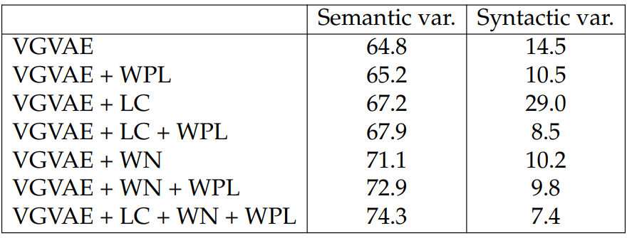
Semantic Similarity. We use cosine similarity between two variables encoded by the inference networks as the predictions and then compute Pearson correlations on the STS Benchmark test set (Cer et al., 2017). As shown in Table 5.8, the semantic variable y always outperforms the syntactic variable z by a large margin, suggesting that different variables have captured different information. Every time when we add WPL the differences in performance between the two variables increases. Moreover, the differences between these two variables are correlated with the performance of models in Table 5.5, showing that a better generation system has a more disentangled latent representation.
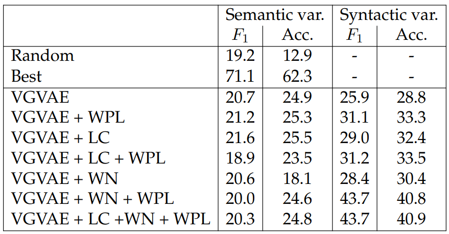
Syntactic Similarity. We use the syntactic evaluation tasks from Section 5.1 to evaluate the syntactic knowledge encoded in the encoder. The tasks are based on a 1- nearest-neighbor constituency parser or POS tagger. To understand the difficulty of these two tasks, Table 5.9 shows results for two baselines. “Random” means randomly pick candidates as predictions. The second baseline (“Best”) is to compute the pairwise scores between the test instances and the sentences in the candidate pool and then take the maximum values. It can be seen as the upper bound performance for these tasks.
As shown in Table 5.9, similar trends are observed as in Tables 5.5 and 5.8. When adding WPL or WN, there is a boost in the syntactic similarity for the syntactic variable. Adding LC also helps the performance of the syntactic variable slightly.
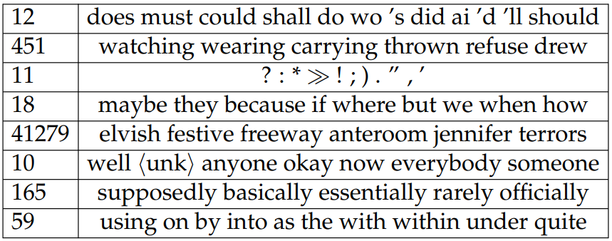
Latent Code Analysis. We look into the learned word clusters by taking the argmax of latent codes and treating it as the cluster membership of each word. Although these are not the exact word clusters we would use during test time (because we marginalize over the latent codes), it provides us intuition on what individual cluster vectors have contributed to the final word embeddings. As shown in Table 5.10, the words in the first and last rows are mostly function words. The second row has verbs. The third row has special symbols. The fourth row also has function words but somewhat different from the first row. The fifth row is a large cluster populated by content words, mostly nouns and adjectives. The sixth row has words that are not very important semantically and the seventh row has mostly adverbs. We also observe that the size of clusters often correlates with how strongly it relates to topics. In Table 5.10, clusters that have size under 20 are often function words while the

largest cluster (5th row) has words with the most concrete meanings.
We also compare the performance of LC by using a single latent code that has 50 classes. The results in Table 5.11 show that it is better to use smaller number of classes for each cluster instead of using a cluster with a large number of classes.
Effect of Decoder Structure. As shown in Fig. 5.6, we evaluate three variants of the decoder, namely INIT, CONCAT, and SWAP. For INIT, we use the concatenation of semantic variable y and syntactic variable z for computing the initial hidden state of decoder and then use the word embedding as input and hidden state to predict the next word. For CONCAT, we move both y and z to the input of the decoder

and use the concatenation of these two variables as input to the decoder and use the hidden state for predicting the next word. For SWAP, we swap the position of y and z to use the concatenation of y and word embeddings as input to the decoder and the concatenation of z and hidden states as output for predicting the next word. Results for these three settings are shown in Table 5.12. INIT performs the worst across the three settings. Both CONCAT and SWAP have variables in each time step in the decoder, which improves performance. SWAP arranges variables in different positions in the decoder and further improves over CONCAT in all metrics.
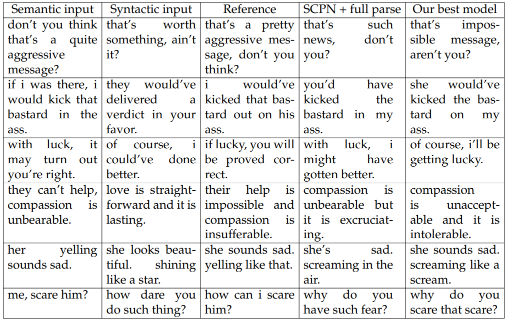
Generated Sentences. We show several generated sentences in Table 5.13. We observe that both SCPN and our model suffer from the same problems. When comparing syntactic input and results from both our models and SCPN, we find that they are always the same length. This can often lead to problems like the first example in Table 5.13. The length of the syntactic input is not sufficient for expressing the semantics in the semantic input, which causes the generated sentences from both models to end at “you?” and omit the verb “think”. Another problem is in the consistency of pronouns between the generated sentences and the semantic inputs. An example is the second row in Table 5.13. Both models alter “i” to be either “you” or “she” while the “kick that bastard in the ass” becomes “kicked the bastard in my ass”.
We found that our models sometimes can generate nonsensical sentences, for example the last row in Table 5.13. while SCPN, which is trained on a much larger corpus, does not have this problem. Also, our models can sometimes be distracted by the word tokens in the syntactic input as shown in the 3rd row in Table 5.13, where our model directly copies “of course” from the syntactic input while since SCPN uses a parse tree, it outputs “with luck”. In some rare cases where the function words in both syntactic inputs and the references are the exactly the same, our models can perform better than SCPN, e.g., the last two rows in Table 5.13. Generated sentences from our model make use of the word tokens “and” and “like” while SCPN does not have access to this information and generates inferior sentences.
This paper is available on arxiv under CC 4.0 license.
